'분류 전체보기' 카테고리의 글 목록

HTTP는 월드 와이드 웹에서 데이터를 전송하기 위한 프로토콜로, 클라이언트와 서버 간에 상호작용하는 데 사용됩니다. HTTP의 특징 중 무상태(stateless)와 상태유지(stateful)에 대해 설명해 드리겠습니다.

1. 무상태(Stateless)
HTTP는 무상태 프로토콜이기 때문에 클라이언트의 상태를 서버가 유지하지 않습니다. 각각의 클라이언트 요청은 독립적으로 처리되며, 이전 요청과 상태 정보를 서버가 알지 못합니다. 서버는 단순히 클라이언트의 요청을 받아들이고 처리한 후 응답을 반환하는 역할만 수행합니다. 클라이언트는 필요한 상태 정보를 요청 매개변수, 헤더 등을 통해 전달해야 합니다.
예를 들어, 사용자가 온라인 상점에서 물건을 구매할 때, 각각의 요청은 주문의 일부분(예: 장바구니에 물건 추가)이나 전체 주문(예: 결제)을 나타내며, 서버는 이전 요청과 상관없이 독립적으로 처리합니다. 클라이언트는 각각의 요청에서 필요한 상품, 수량 및 주소 정보를 제공하여 서버가 요청을 처리할 수 있도록 해야 합니다.

2. 상태유지(Stateful)
반면에, 상태유지 프로토콜은 서버가 클라이언트의 상태 정보를 유지합니다. 서버는 클라이언트가 연결된 상태를 추적하고 클라이언트의 요청에 따라 이전의 상태를 기반으로 응답합니다. 서버는 클라이언트의 상태 정보를 세션, 쿠키, 데이터베이스 등을 사용하여 저장합니다.
예를 들어, 인터넷 뱅킹 서비스에서 사용자가 로그인하면, 서버는 사용자의 인증 정보를 기반으로 클라이언트와의 세션을 설정합니다. 이후 클라이언트가 다른 요청을 보낼 때마다 서버는 세션 정보를 사용하여 해당 사용자의 상태를 파악하고, 예를 들어 잔액 조회, 계좌 이체 등의 서비스를 제공합니다.

요약하면, HTTP는 기본적으로 무상태 프로토콜이지만, 필요에 따라 상태유지를 위한 기능들을 사용할 수 있습니다.

저작자표시 비영리 (새창열림)

input 태그 속성에 onKeyup="this.value=this.value.replace(/[^0-9]/g,'');" 를 추가해주면 된다.

저작자표시 비영리 (새창열림)

'Web > HTML | JSP' 카테고리의 다른 글

쿠키와 세션비교 (0)	2021.06.02

on( )

jQuery는 특정 요소에 이벤트 바인딩(event binding)하기 위해 .on()를 사용한다.

(bind() 대신 사용 가능)

기본형

$("p").on("click", function(){
 alert("문장이 클릭되었습니다.");
});

이벤트 핸들러 하나에 이벤트를 여러개 설정

$("p").on("mouseenter mouseleave", function() {
  $("div").append("마우스 커서가 문장 위로 들어오거나 빠져 나갔습니다.<br>");
});

또한, 하나의 요소에 여러 개의 이벤트 핸들러를 사용하여 여러 개의 이벤트를 같이 바인딩할 수도 있다.

$("p").on({ 
  click: function() {
    $("div").append("마우스가 문장을 클릭했습니다.<br>");
  },
  mouseenter: function() {
    $("div").append("마우스가 커서가 문장 위로 들어왔습니다.<br>");
  },
  mouseleave: function() {
    $("div").append("마우스가 커서가 문장을 빠져 나갔습니다.<br>");
  }
});

off( )

.off()는 더 이상 사용하지 않는 이벤트와의 바인딩(binding)을 제거한다.

$("#btn").on("click", function() {
  alert("버튼을 클릭했습니다.");
});
$("#btnBind").on("click", function() {
  $("#btn").on("click").text("버튼 클릭 가능");
});
$("#btnUnbind").on("click", function() {
  $("#btn").off("click").text("버튼 클릭 불가능");
});

one( )

one()는 바인딩(binding)된 이벤트 핸들러가 한번만 실행되고 나서는, 더는 실행되지 않는다.

$("button").one("click", function() {
  $("div").append("이제 클릭이 되지 않습니다.<br>");
});

저작자표시 비영리 (새창열림)

'Web > 자바스크립트' 카테고리의 다른 글

querySelector() / querySelectorAll() 사용법 (0)	2022.03.29
innerText / innerHTML 비교 (0)	2022.03.29
[javascript] var hoisting (0)	2021.05.27
[javascript] use strict (strict mode) (0)	2021.05.26
[javascript] asyn, defer 비교 (0)	2021.05.26

querySelector

dom 요소를 하나만 선택할 때 사용한다.

해당 요소의 속성을 변경하거나, 자식 / 부모 관계로 Element를 만들 때 주로 사용된다.

예제1

<!doctype html>
<html lang="ko">
  <head>
    <meta charset="utf-8">
    <title>JavaScript</title>
  </head>
  <body>
    <p class="abc">Lorem Ipsum Dolor</p>
    <p class="abc">Lorem Ipsum Dolor</p>
    <p class="abc">Lorem Ipsum Dolor</p>
    <script>
      document.querySelector( '.abc' ).style.color = 'red';
    </script>
  </body>
</html>

예제2

<!doctype html>
<html lang="ko">
  <head>
    <meta charset="utf-8">
    <title>JavaScript</title>
  </head>
  <body>
    <p class="abc">Lorem Ipsum Dolor</p>
    <div>
      <p class="abc">Lorem Ipsum Dolor</p>
      <p class="abc">Lorem Ipsum Dolor</p>
    </div>
    <script>
      document.querySelector( 'div .abc' ).style.color = 'red';
    </script>
  </body>
</html>

querySelectorAll

해당되는 모든 요소를 nodeList(배열)로 반환한다.

예제1

<!doctype html>
<html lang="ko">
  <head>
    <meta charset="utf-8">
    <title>JavaScript</title>
  </head>
  <body>
    <p class="abc">Lorem Ipsum Dolor</p>
    <p class="abc">Lorem Ipsum Dolor</p>
    <p class="abc">Lorem Ipsum Dolor</p>
    <script>
      var jb = document.querySelectorAll( '.abc' );
      jb[1].style.color = 'red';
    </script>
  </body>
</html>

예제2

<!doctype html>
<html lang="ko">
  <head>
    <meta charset="utf-8">
    <title>JavaScript</title>
  </head>
  <body>
    <p class="abc">Lorem Ipsum Dolor</p>
    <p class="abc">Lorem Ipsum Dolor</p>
    <p class="abc">Lorem Ipsum Dolor</p>
    <script>
      var jb = document.querySelectorAll( '.abc' );
      for ( var i = 0; i < jb.length; i++ ) {
        jb[i].style.color = 'red';
      }
    </script>
  </body>
</html>

저작자표시 비영리 (새창열림)

'Web > 자바스크립트' 카테고리의 다른 글

jquery 이벤트 처리 on() / off() / one() (0)	2022.03.30
innerText / innerHTML 비교 (0)	2022.03.29
[javascript] var hoisting (0)	2021.05.27
[javascript] use strict (strict mode) (0)	2021.05.26
[javascript] asyn, defer 비교 (0)	2021.05.26

값 가져오기 (innerText vs innerHTML)

이 두 속성은 다루는 값이 text element인지, html element인지에 따라 사용법이 다르다.

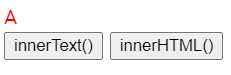
<div id='content'>
  <div>A</div>
  <div>B</div>
</div>

<input 
  type='button' 
  value='innerText()'
  onclick='getInnerText()' />
<input 
  type='button' 
  value='innerHTML()' 
  onclick='getInnerHTML()' />

function getInnerText()  {
  const element = document.getElementById('content');
  alert(element.innerText);
  // A
  // B
}

function getInnerHTML()  {
  const element = document.getElementById('content');
  alert(element.innerHTML);
  // <div>A</div>
  // <div>B</div>
}

element.innerText;

이 속성은 element 안의 text 값들만을 가져옵니다.

element.innerHTML;

innerText와는 달리 innerHTML은 element 안의 HTML이나 XML을 가져옵니다.

값 설정하기 (innerText vs innerHTML)

<div id='content'>
</div>

<input 
  type='button' 
  value='innerText()'
  onclick='setInnerText()' />
<input 
  type='button' 
  value='innerHTML()' 
  onclick='setInnerHTML()' />

function setInnerText()  {
  const element = document.getElementById('content');
  element.innerText = "<div style='color:red'>A</div>";
} 
// <div style='color:red'>A</div>



function setInnerHTML()  {
  const element = document.getElementById('content');
  element.innerHTML = "<div style='color:red'>A</div>";
}
// A

<- innerText() 버튼 클릭

<- innerHTML() 버튼 클릭

element.innerText = "<div style='color:red'>A</div>";

element.innerText에 html을 포함한 문자열을 입력하면,

html코드가 문자열로 element안에 포함되어 문자열이 html 코드라도 html코드로서 적용이 되지 않는다.

(단순한 문자열로 해당 element 안에 삽입)

element.innerHTML = "<div style='color:red'>A</div>";

위와 같이 element.innerHTML 속성에 html코드를 입력하면,

html 코드가 적용이 되어 해당 element 안에 적용 된다.

위 예제에서 'innerHTML()'을 클릭하면,

입력된 html태그가 해석되어 빨간색A 가 나타나는 것을 확인 할 수 있다.

저작자표시 비영리 (새창열림)

'Web > 자바스크립트' 카테고리의 다른 글

jquery 이벤트 처리 on() / off() / one() (0)	2022.03.30
querySelector() / querySelectorAll() 사용법 (0)	2022.03.29
[javascript] var hoisting (0)	2021.05.27
[javascript] use strict (strict mode) (0)	2021.05.26
[javascript] asyn, defer 비교 (0)	2021.05.26

AOP(Aspect Oriented Programming)는 관점지향프로그래밍이라고 불린다. 관점지향은 어떤 로직을 기준으로 핵심적인 관점, 부가적인 관점으로 나누어서 보고 그 관점을 기준으로 각각 모듈화하겠다는 것이다. 여기서 모듈화란 어떤 공통된 로직이나 기능을 하나의 단위로 묶는 것을 말한다.

핵심적인 관점은 핵심 비즈니스 로직을 의미하고 부가적인 관점은 핵심로직을 실행하기 위해 행해지는 DB연결, 로깅, 예외처리 등이 있다. 소스코드 상에서 다른 부분에 반복해서 쓰는 코드들이 있는데 이것을 흩어진 관심사라고 부른다. 여기서 이 흩어진 관심하를 모듈화하고 핵심적인 비즈니스 로직에서 분리하여 재사용하겠다는 것이 AOP의 취지이다.

AOP의 주요 개념

- Aspect : 흩어진 관심사를 모듈화 한 것 (부가기능을 모듈화 한 것)

- Target : Aspect를 적용하는 곳(클래스, 메서드...) [부가기능을 부여할 대상]

- Advice : 실질적으로 부가기능을 담은 구현체 / Advice는 Aspect가 무엇을 언제 할지를 정의한다.

- JoinPoint : Advice가 적용될 수 있는 위치

- PointCut : JoinPoint의 상세한 스펙을 정의하여 선별 / 구체적으로 Advice가 실행될 지점을 정함 (ex : A라는 메서드의 진입 시점에 호출할 것)

- Proxy : 타겟을 감싸서 타겟의 요청을 대신 받아주는 랩핑 오브젝트

- Introduction : 타겟 클래스에 코드 변경없이 신규 메소드나 멤버변수를 추가하는 기능

- Weaving : 지정된 객체에 애스팩트를 적용해서 새로운 프록시 객체를 생성하는 과정

저작자표시 비영리 (새창열림)

데이터 분석을 위해 파이썬에서는 Pandas와 Numpy 그리고 Matplotlib를 제공한다. 이 글에서는 matplotlib 을 사용해 보겠다. matplotlib는 python에서 다양한 시각화 기술을 구현하는 라이브러리이다.

먼저 matplotlib을 사용하기 위해서는 아래와 같이 import 선언을 해주어야 한다.

필자는 matplotlib패키지의 pyplot모듈을 사용하기 위해 plt라는 객체명을 선언하였다.

import matplotlib.pyplot as plt

numpy를 사용하여 배열을 먼저 생성해보자

import numpy as np

x = np.arange(-4.5, 5, 0.5)
y = 2 * x ** 2
[x,y]

->
[array([-4.5, -4. , -3.5, -3. , -2.5, -2. , -1.5, -1. , -0.5,  0. ,  0.5,
         1. ,  1.5,  2. ,  2.5,  3. ,  3.5,  4. ,  4.5]),
 array([40.5, 32. , 24.5, 18. , 12.5,  8. ,  4.5,  2. ,  0.5,  0. ,  0.5,
         2. ,  4.5,  8. , 12.5, 18. , 24.5, 32. , 40.5])]

show() - 그래프 그리기

위 생성된 배열을 각각 x, y 값으로 그래프로 표현해보자

plt.plot(x,y)
plt.show()

figure(), subplot()

x = np.arange(-4.5, 5, 0.5)
y1 = 2*x**2
y2 = 5*x + 30
y3 = 4*x**2 + 10

plt.plot(x, y1)
plt.plot(x, y2)
plt.plot(x, y3)
plt.show()

plt.plot(x, y1)

plt.figure()
plt.plot(x,y2)

plt.show()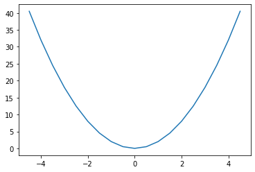

x = np.arange(-5, 5, 0.1)
y1 = x**2 -2
y2 = 20 * np.cos(x)**2

plt.figure(1) #1번 그래프 창 생성
plt.plot(x, y1)
plt.figure(2) #2번 그래프 창 생성
plt.plot(x, y2)
plt.figure(1) # 이미 생성된 1번 그래프 창을 지정
plt.plot(x, y2)
plt.figure(2) #이미 생성된 2번 그래프 창을 지정
plt.clf() # 2번 그래프 창에 그려진 모든 그래프를 지움
plt.plot(x,y1) #지정된 그래프 창에 그래프를 그림
plt.show()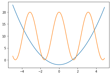

x = np.arange(0, 10, 0.1)
y1 = 0.3*(x-5)**2 + 1
y2 = -1.5*x +3
y3 = np.sin(x)**2
y4 = 10*np.exp(-x) + 1

# 2x2 행렬로 이루어진 서브 그래프에서 p에 따라 위치를 지정
plt.subplot(2,2,1) # p는 1
plt.plot(x,y1)
plt.subplot(2,2,2) # p는 2
plt.plot(x,y2)
plt.subplot(2,2,3) # p는 3
plt.plot(x,y3)
plt.subplot(2,2,4) # p는 4
plt.plot(x,y4)
plt.show()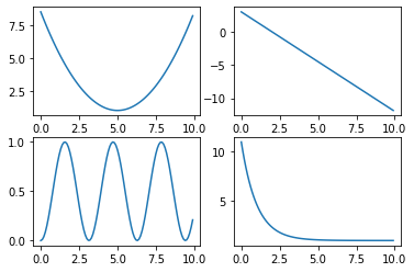

xlim(), xlim() - 그래프의 x축, y축의 범위 설정

x = np.linspace(-4, 4, 100)
y1 = x**3
y2 = 10*x**2 -2

plt.plot(x,y1,x,y2)
plt.xlim(-1,1) # x축의 범위를 -1에서 1로 한정
plt.ylim(-3,3) # y축의 범위를 -3에서 3로 한정
plt.show()

그래프 그리기 예시

import matplotlib

matplotlib.rcParams['font.family'] = 'Malgun Gothic'
matplotlib.rcParams['axes.unicode_minus'] = False

plt.plot(x, y1, '>--r', x, y2, 's-g', x, y3, 'd:b', x, y4, '-.Xc')
plt.legend(['데이터1', '데이터2', '데이터3', '데이터4'], loc = 'best')
plt.xlabel('X 축')
plt.ylabel('Y 축')
plt.title('그래프 제목')
plt.grid(True)

import matplotlib.pyplot as plt

height = [165,177,160,180,185,155,172]
weight = [62,67,55,74,90,43,64]

plt.scatter(height, weight)
plt.xlabel('Height(m)')
plt.ylabel('Weight(Kg)')
plt.title('Height & Weight')
plt.grid(True)

plt.scatter(height, weight, s=500, c='r')
plt.show()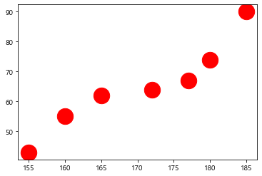

city = ['서울', '인천', '대전', '대구', '울산', '부산', '광주']
# 위도(latitude)와 경도(longitude)
lat = [37.56,37.45,36.35,35.87,35.53,35.18,35.16]
lon = [126.97,126.70,127.38,128.60,129.31,129.07,126.85]
#인구 밀도(명/km^2): 2017년 통계청 자료
pop_den = [16154,2751,2839,2790,1099,4454,2995]

size = np.array(pop_den) * 0.2 # 마커의 크기 지정
colors = ['r', 'g', 'b', 'c', 'm', 'k', 'y'] # 마커의 컬러지정
plt.scatter(lon, lat, s=size, c=colors, alpha=0.5)
plt.xlabel('경도(longitude)')
plt.ylabel('위도(latitude)')
plt.title('지역별 인구 밀도(2017)')

for x, y, name in zip(lon, lat, city):
    plt.text(x, y, name) # 위도 경도에 맞게 도시 이름 출력
plt.show()

member_IDs = ['m_01', 'm_02', 'm_03', 'm_04']
before_ex = [27, 35, 40, 33]
after_ex = [30,38,42,37]

n_data = len(member_IDs)
index = np.arange(n_data)
plt.bar(index, before_ex)
plt.show()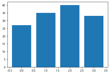

barWidth = 0.4
plt.bar(index, before_ex, color='c', align='edge', width = barWidth, label='before')
plt.bar(index + barWidth, after_ex, color='m', align='edge', width = barWidth, label='after')

plt.xticks(index + barWidth, member_IDs)
plt.legend()
plt.xlabel('회원 ID')
plt.ylabel('위몸일으키기 횟수')
plt.title('운동 시작 전과 후의 근지구력(복근) 변화 비교')
plt.show()

fruit = ['사과', '바나나', '딸기', '오렌지', '포도']
result = [7,6,3,2,2]

plt.pie(result)
plt.show()

plt.figure(figsize=(5,5))
plt.pie(result, labels = fruit, autopct='%.1f%%')
plt.show()

explode_value = (0.1,0,0,0,0)

plt.figure(figsize=(5,5))
plt.pie(result, labels=fruit, autopct='%.1f%%', startangle=90, counterclock=False, explode=explode_value, shadow=True)
plt.show()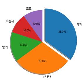

import pandas as pd

temperature = [25.2,27.4,22.9,26.2,29.5,33.1,30.4,36.1,34.4,29.1]
Ice_cream_sales = [236500,357500,203500,365200,446600,574200,453200,675400,598400,463100]

dict_data = {'기온':temperature, '아이스크림 판매량':Ice_cream_sales}
df_ice_cream = pd.DataFrame(dict_data, columns=['기온', '아이스크림 판매량'])
df_ice_cream

df_ice_cream.plot.scatter(x='기온', y='아이스크림 판매량', grid=True, title='최고 기온과 아이스크림 판매량')
plt.show()

matplotlib-1.html

1.07MB

wordcloud를 이용한 데이터 통계

import pandas as pd

word_count_file = "C:/pywork/word_count.csv"
word_count = pd.read_csv(word_count_file, index_col = '단어')
word_count.head(5)

->
	빈도
단어	
산업혁명	1662
기술	1223
사업	1126
혁신	1084
경제	1000

from wordcloud import WordCloud
import matplotlib.pyplot as plt

korean_font_path = 'C:/Windows/Fonts/malgun.ttf'

wc = WordCloud(font_path=korean_font_path, background_color='white')

frequencies = word_count['빈도'] # pandas의 Series 형식
wordcloud_image = wc.generate_from_frequencies(frequencies)

wc = WordCloud(font_path=korean_font_path, background_color='white')

frequencies = word_count['빈도'] # pandas의 Series 형식
wordcloud_image = wc.generate_from_frequencies(frequencies)

matplotlib-2.html

0.61MB

저작자표시 비영리 (새창열림)

'Python' 카테고리의 다른 글

[Python] Pandas 사용 (0)	2021.07.28
[Python] Numpy 사용 (0)	2021.07.27
[Python] 명령문으로 파일 생성, 작성, 읽어오기 (0)	2021.07.27
jupyter notebook 에서 Python 파일 생성 / 폴더(directory) 생성 방법 (0)	2021.07.27
[Python] split(), strip(), find(), startswith(), endswith(), replace(), isalnum(), isspace() 함수 (0)	2021.07.27

데이터 분석을 위해 파이썬에서는 Pandas와 Numpy 그리고 Matplotlib를 제공한다. 이 글에서는 pandas의 함수사용법에 대해 알아보겠다. pandas는 파이썬의 데이터 처리를 위한 라이브러리이다.

pandas를 사용하기 위해서는 pandas모듈을 import를 해야한다. 보통 pd라는 별칭으로 사용한다.

import pandas as pd
import numpy as np

Series() - 시리즈는 1차원 배열의 값(values)에 각 값에 대응되는 인덱스(index)를 부여할 수 있는 구조를 갖는다

s5 = pd.Series({'국어':100, '영어':95, '수학':90})
s5
->
국어    100
영어     95
수학     90
dtype: int64

index_date = ['2018-10-07', '2018-10-08', '2018-10-09', '2018-10-10']
s4 = pd.Series([200, 195, np.nan, 205], index = index_date)
s4

->
2018-10-07    200.0
2018-10-08    195.0
2018-10-09      NaN
2018-10-10    205.0
dtype: float64

date_range() - 날짜 범위 만들기

(freq='D'로 선언하면 day를 기준으로 날짜를 나누겠다는 뜻 -> periods=5로 선언되어 있으므로 시작날짜 2021-02-01부터 5일을 부여하겠다는 의미 / freq는 생략 가능한데 생략할 시 default 값은 'D'(day))

index_date = pd.date_range(start = '2021-02-01', periods = 5, freq='D')
pd.Series([51,62,55,49,58], index = index_date)

->
2021-02-01    51
2021-02-02    62
2021-02-03    55
2021-02-04    49
2021-02-05    58
Freq: D, dtype: int64

DataFrame() - 2차원 데이터 테이블 구조를 가지는 자료형.

데이터프레임은 2차원 리스트를 매개변수로 전달한다. 2차원이므로 행방향 인덱스(index)와 열방향 인덱스(column)가 존재한다. 즉, 행과 열을 가지는 자료구조이다. 시리즈가 인덱스(index)와 값(values)으로 구성된다면, 데이터프레임은 열(columns)까지 추가되어 열(columns), 인덱스(index), 값(values)으로 구성된다.

data = np.array([[1,2,3], [4,5,6], [7,8,9], [10,11,12]])
index_date = pd.date_range('2019-09-01', periods=4)
columns_list = ['A', 'B', 'C']
pd.DataFrame(data, index=index_date, columns=columns_list)

->
		A	B	C
2019-09-01	1	2	3
2019-09-02	4	5	6
2019-09-03	7	8	9
2019-09-04	10	11	12

table_data3 = {'봄': [256.5,264.3,215.9,223.2,312.8],
              '여름': [770.6,567.5,599.8,387.1,446.2],
              '가을': [363.5,231.2,293.1,247.7,381.6],
              '겨울': [139.3,59.9,76.9,109.1,108.1]}
columns_list = ['봄', '여름', '가을', '겨울']
index_list = ['2012', '2013', '2014', '2015', '2016']

df3 = pd.DataFrame(table_data3, columns = columns_list, index = index_list)
df3

->
	봄	여름	가을	겨울
2012	256.5	770.6	363.5	139.3
2013	264.3	567.5	231.2	59.9
2014	215.9	599.8	293.1	76.9
2015	223.2	387.1	247.7	109.1
2016	312.8	446.2	381.6	108.1

mean() - 평균 구하기 (axis=1 이면, 행 기준)

df3.mean()
->
봄     254.54
여름    554.24
가을    303.42
겨울     98.66
dtype: float64

df3.mean(axis=1)
->
2012    382.475
2013    280.725
2014    296.425
2015    241.775
2016    312.175
dtype: float64

describe() - 데이터 요약

df3.describe()
->
	봄		여름		가을		겨울
count	5.000000	5.000000	5.000000	5.000000
mean	254.540000	554.240000	303.420000	98.660000
std	38.628267	148.888895	67.358496	30.925523
min	215.900000	387.100000	231.200000	59.900000
25%	223.200000	446.200000	247.700000	76.900000
50%	256.500000	567.500000	293.100000	108.100000
75%	264.300000	599.800000	363.500000	109.100000
max	312.800000	770.600000	381.600000	139.300000

데이터 조회

KTX_data = {'경부선 KTX': [39060,39896,42005,43621,41702,41266,32427],
            '호남선 KTX': [7313,6967,6873,6626,8675,10622,9228],
            '경전선 KTX': [3627,4168,4088,4424,4606,4984,5570],
            '전라선 KTX': [309,1771,1954,2244,3146,3945,5766],
            '동해선 KTX': [np.nan,np.nan,np.nan,np.nan,2395,3786,6667]}
col_list = ['경부선 KTX', '호남선 KTX', '경전선 KTX', '전라선 KTX', '동해선 KTX']
index_list = ['2011', '2012', '2013', '2014', '2015', '2016', '2017']

df_KTX = pd.DataFrame(KTX_data, columns = col_list, index = index_list)
df_KTX

행 기준 indexing

df_KTX[1:2]

index 또는 column 명으로 조회

df_KTX.loc['2013':'2016']

df_KTX['경부선 KTX']['2012':'2014']

->
2012    39896
2013    42005
2014    43621
Name: 경부선 KTX, dtype: int64

.T - 행과 열 바꾸기

df_KTX.T # T -> 행과 열 바꾸기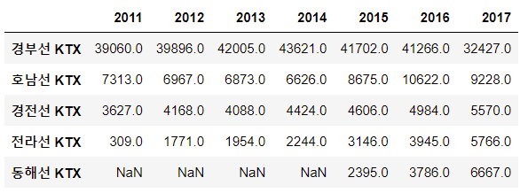

append() - 테이블 붙이기

(ignore_index=True 일 경우 붙임 당하는 테이블의 index를 이어서 적용한다 (속성 생략 가능))

df1 = pd.DataFrame({'Class1':[95,92,98,100],
                    'Class2':[91,93,97,99]})
df1

->
	Class1	Class2
0	95	91
1	92	93
2	98	97
3	100	99

df2 = pd.DataFrame({'Class1': [87,89],
                   'Class2': [85,90]})
df2

->
	Class1	Class2
0	87	85
1	89	90

df1.append(df2, ignore_index=True)

->
	Class1	Class2
0	95	91
1	92	93
2	98	97
3	100	99
4	87	85
5	89	90

join() - 테이블 합치기

index_label = ['a','b','c','d']
df1a = pd.DataFrame({'Class1':[95,92,98,100],
                    'Class2':[91,93,97,99]}, index=index_label)
df5 = pd.DataFrame({'Class4':[82,92]})
df1.join(df5)

->
	Class1	Class2	Class4
0	95	91	82.0
1	92	93	92.0
2	98	97	NaN
3	100	99	NaN

merge() - 테이블 결합

df_left = pd.DataFrame({'key':['A','B','C'], 'left':[1,2,3]})
df_left

->
	key	left
0	A	1
1	B	2
2	C	3

df_right = pd.DataFrame({'key':['A','B','D'], 'right':[4,5,6]})
df_right

->
	key	right
0	A	4
1	B	5
2	D	6

#df_left를 기준(how='left')(df_left가 merge왼쪽에 있으므로)을 두고 on='key'에서 속성 값인 key(컬럼)를 비교하여 key(컬럼)가 일치하거나 left의 key만 있는경우 결합

df_left.merge(df_right, how='left', on='key') 

->
	key	left	right
0	A	1	4.0
1	B	2	5.0
2	C	3	NaN

#df_right를 기준(how='right')(df_right가 merge오른쪽에 있으므로)을 두고 on='key'에서 속성 값인 key(컬럼)를 비교하여 key(컬럼)가 일치하거나 right의 key만 있는경우 결합

df_left.merge(df_right, how='right', on='key') 

->
	key	left	right
0	A	1.0	4
1	B	2.0	5
2	D	NaN	6

df_left.merge(df_right, how='outer', on='key') 

->
	key	left	right
0	A	1.0	4.0
1	B	2.0	5.0
2	C	3.0	NaN
3	D	NaN	6.0

df_left.merge(df_right, how='inner', on='key')

->
	key	left	right
0	A	1	4
1	B	2	5

pandas.html

0.66MB

저작자표시 비영리 (새창열림)

'Python' 카테고리의 다른 글

[Python] Matplotlib사용 (0)	2021.07.28
[Python] Numpy 사용 (0)	2021.07.27
[Python] 명령문으로 파일 생성, 작성, 읽어오기 (0)	2021.07.27
jupyter notebook 에서 Python 파일 생성 / 폴더(directory) 생성 방법 (0)	2021.07.27
[Python] split(), strip(), find(), startswith(), endswith(), replace(), isalnum(), isspace() 함수 (0)	2021.07.27

기억보단 기록을